Control Loops¶

Control loops are software used to operate power transmission systems (such as a drivetrain or linear slide) in a fast and controlled fashion. Not only do control loops let you run mechanisms quickly without fear of losing control, in many cases, they help preserve the longevity of mechanisms by reducing rapid change of applied motor voltage.

What is Error?¶

The first thing that must be defined when discussing control loops is the concept of error. Error is defined as the difference between where you are and where you want to be. For instance, say you tell your drivetrain to drive at 30 inches per second, but in actuality, at a time, the drivetrain is driving at 28 inches per second. Since $30-28=2$ , the error of the drivetrain’s speed at this time $T$ is 2 inches per second. In other words, at a time $t=T$ , $e(t)=2$ .

PID¶

A PID controller (or Proportional Integral Derivative controller) is a control loop that solely uses error to control the system. PID is a form of a feedback control loop, or closed loop control. This means that data about the variable you are controlling is required in order for the loop to control that variable. In this case, information about the error of the system is required to control the system with a PID controller.

The Optional Calculus¶

The following equation represents the rigorous mathematical definition of the output of a PID controller $f$ at any given time $t$ :

$f(t) = K_p e(t) + K_i \int_o^t e(t) \mathrm{d}t + K_d \frac{\mathrm{d}e(t)}{\mathrm{d}t}$

where $K_p$ , $K_i$ , and $K_d$ are constants and $e(t)$ , as previously mentioned, is the error in the system. If you have no experience with calculus, don’t worry; while PID is fundamentally rooted in calculus, you do not need any calculus experience to be able to understand it, only basic algebra. However, you are still urged to read the rest of the section regardless of calculus experience, as the formula alone doesn’t tell you why it works.

Simplification of the PID formula¶

Here is a simplified version of the PID formula: $f(t)=K_p P(t)+K_i I(t)+K_d D(t)$

All we have done is simply take the full formula and replaced part of the terms with functions: $P(t)$ , $I(t)$ , and $D(t)$ .

The Proportional Term¶

The first component of the function, $K_p P(t)$ , is by far the most simple and easy to understand, as $P(t) = e(t)$ . For the sake of example, let’s pretend that $K_i=0$ and $K_d=0$ (a PID controller with only a proportional constant is known as a P controller). How will the system behave? Well, if the error is large, the output will be large. Likewise, if the error is small, the output will be small. Also, ideally, given enough time, the system always approaches its destination, assuming $K_p$ is of the correct sign.

Say we apply this to a drivetrain. You want to drive a distance $D$ , and you decide to set your motor powers using a P controller to accomplish this. In this case, your error is how far away the robot is from the desired location. As you start to drive forward, your error is large, so you drive forward quickly, which is desirable. After all, you aren’t concerned with overshooting the target yet if you are far away from it. But as the robot’s distance to the target approaches 0, you will start to slow down, gaining more control over the robot. Once the error is zero, ideally, the robot will stop, and you have reached your destination. If you happen to overshoot, the error will become negative, and the robot will backtrack, repeating the process.

The Derivative Term¶

This term, $K_d D(t)$ , is intended to dampen the rate of change of the error. In other words, it tries to keep the error constant. How is this done? Well, for those of you with calculus under your belt, $D(t)=\frac{de(t)}{dt}$ . For those without calculus experience, it represents how fast the error is changing. Graphically, $D(t)$ is simply the slope of the error at any given time $t$ . This slope can be calculated by keeping track of the error over successive iterations of the control loop. One iteration occurs at time $t_n$ with an error of $e(t_n)$ . At the next iteration, the time is $t_{n+1}$ with an error of $e(t_{n+1})$ . Thus, to find $D(t)$ , simply find the slope of $e(t)$ given these two points.

The Integral Term¶

Admittedly, the integral term is the least important term for FTC PID control loops. With a properly tuned $K_p$ and $K_d$ , you often can just set $K_i$ to 0 and call it a day. However, it can still be useful in some cases. Just like the derivative term, the integral term intends to correct for overshoot. if the system thinks it reached its destination, it will stop, even when, in fact, the error is not yet 0. Perhaps the motor is no longer being supplied enough power to move. Well, given enough time, the integral term will increase the output (in this case, motor power), causing movement towards the destination. To explain without calculus, the integral term essentially sums the error over a specific interval of time. To do this, error in each loop iteration is added to a variable (in this case, $I(t)$ ). However, summing error this way has an unfortunate side effect: the longer the loop takes to complete one iteration, the more slowly this sum increases, which is obviously not desirable, as we don’t want lag to affect how the robot moves. To compensate for this, before the error is added to $I(t)$ , it is multiplied by how long the previous loop took to-complete, or $t_{n+1}-t_n$ , preventing lag from making the system sum more slowly.

So say the robot stops short of the target. The P and D combination aren’t strong enough to move it forward to the destination. You can either tune $K_p$ and $K_d$ to compensate (this is recommended), or you can add the integral term to increase output (this works too, but requires more attention and tuning to achieve the same result).

PID Pseudocode¶

while True:
    current_time = get_current_time()
    current_error = desire_position-current_position

    p = k_p * current_error

    i += k_i * (current_error * (current_time - previous_time))

    if i > max_i:
        i = max_i
    elif i < -max_i:
        i = -max_i

    D = k_d * (current_error - previous_error) / (current_time - previous_time)

    output = p + i + d

    previous_error = current_error
    previous_time = current_time

Tuning a PID Loop¶

The most important thing to know while tuning a PID loop is how each of the terms affects the output. This can allow you to see which gains need to be adjusted. For example, if the target is not reached but instead the setpoint begins to oscillate around the target, it means there is not enough D gain. If the target is eventually reached, albeit very slowly, that means there is not enough P gain or the D gain is too high. In brief, the P variable drives the error towards zero, the I variable corrects for steady state error, and the D variable dampens the effects of the P variable, more so as error approaches zero, which prevents overshoot.

The most common method for tuning a PID controller is as follows:

Set the I and D gains to zero
Increase the P gain until there are oscillations around the target
Increase the D gain until no overshoot occurs
If there is steady state error, increase the I gain until it is corrected

An important thing to note is that most systems do not need both I and D control. Generally, systems without a lot of friction do not need an I term, but will need more D control. Systems with a lot of friction, on the other hand, generally do not need D control because the friction facilitates deceleration but need I control because the friction prevents the system from reaching the target otherwise.

For a more in-depth explanation, click here

Feedforward Control¶

One less popular but equally useful control loop is the feedforward controller (sometimes unofficially referred to in FTC as the PVA controller, or Position-Velocity-Acceleration controller). For those without a physics background, velocity is the speed and direction something is moving and acceleration is how fast velocity is increasing or decreasing. Unlike PID, feedforward controllers require you to input not only where you want to go and where you are, but how fast you want to be moving at all times. Unlike feedback control loops such as PID, feedforward control loops don’t require information about the variable you want to control. Instead of controlling a variable directly, it controls how fast that variable changes.

Conceptually, the controller is made up of 2 separate P controllers (remember, a P controller is made up of just the proportional term of a PID loop). Each of these P controllers are added together to create a feedforward controller.

Just like we did with the PID formula, we can define the function like this: $f(t)=K_v*V(t)+K_a*A(t)$ .

In most FTC applications, $f(t)$ controls the position of the output. As the name PVA suggests, the first term relates to velocity, and the second relates to acceleration. Just like in a P controller, each term contains a constant multiplied by an error term (in this case, $V(t)$ and $A(t)$ ). However, unlike a PID controller, each term has their own setpoints and endpoints, meaning error is calculated differently for each term.

Unlike desired position, your desired velocity is likely to change throughout the control loop. After all, the entire point of using control loops are to try to create a balance of speed and control of a system. Remember, in most situations, you want to approach your destination quickly if you are far away and slow down if you are close for more control. For the sake of example, let’s say $v(t)$ is a magic function that could tell you exactly how fast you should be going at any point. To calculate velocity error, subtract your current velocity from the magic function $v(t)$ . This magic function can also be used to create another magic function: $a(t)$ . This magic function tells you how exactly how fast the velocity should change in order to get to the next magic velocity at any specified time.

The last step is finding the magic functions $v(t)$ and $a(t)$ , which can be obtained using motion profiles (discussed next).

Feedforward Pseudocode¶

while True:
    current_time = get_current_time()

    current_velocity = (current_position - previous_position) / (current_time - previous_time)
    current_velocity_error = desired_velocity - current_velocity

    current_acceleration = (current_velocity - previous_velocity) / (current_time - previous_time)
    current_acceleration_error = desired_acceleration - current_acceleration
    output = F + k_v * current_velocity_error + K_A * current_acceleration_error

    previous_velocity = current_velocity

    # end of feedforward code

    previous_error = current_error
    previous_time = current_time

Motion Profiles¶

Motion profiling is a technique popularized in FRC that is starting to find its way to FTC. A motion profile is a function used to change the speed of a power transmission system in a controlled and consistent way by changing desired speed gradually rather than instantaneously. Let’s illustrate this with an example: say you want your drivetrain, which is initially unmoving, to drive forward at full speed. Ordinarily, you would set all drivetrain motors to full power in the code. However, this can be problematic because even though you tell the motors to move at full speed instantaneously, the drivetrain takes time to get to full speed. This can lead to uncontrolled movements which have the potential to make autonomous less consistent and, perhaps more importantly, damage mechanisms. Motion profiling attempts to solve this issue.

Advantages¶

More controlled and predictable movements
Reduces rapid change of applied motor voltage

Disadvantages¶

Can be slower

There are two main types of motion profiles: Trapezoidal profiles and S-Curve profiles. Trapezoidal profiles accelerate the system at a constant rate, and S-Curve profiles assume jerk (the speed acceleration changes) is constant. Given that S-Curve profiles are not optimal for controlling 2d trajectories (such as driving) and exist to reduce slippage (which usually only occurs when driving in FTC), trapezoidal profiles are recommended for most FTC applications.

Trapezoidal profiles get their name from the shape of the graph of velocity over time:

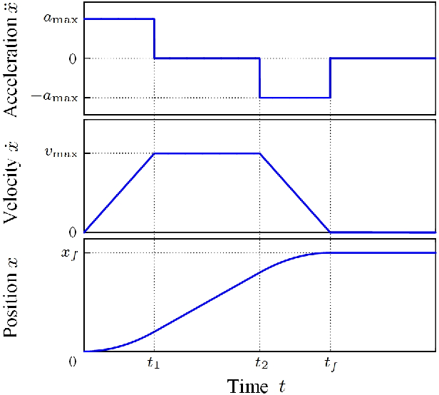
These are the “magic functions” for velocity and acceleration over time alluded to in the feedforward section.¶

Here is some pseudocode for a trapezoidal profile:

while True:
    current_velocity = get_current_velocity()
    current_time = get_current_time()

    direction_multiplier = 1

    if position_error < 0:
        direction_multiplier = -1

    # if maximum speed has not been reached
    if MAXIMUM_SPEED > abs(current_velocity):
        output_velocity = current_velocity + direction_multiplier * MAX_ACCELERATION * (current_time - previous_time)
        output_acceleration = MAX_ACCELERATION

    #if maximum speed has been reached, stay there for now
    else:
        outputVelocity = MAXIMUM_SPEED
        outputAcceleration = 0

    #if we are close enough to the object to begin slowing down
    if position_error <= (output_velocity * output_velocity) / (2 * MAX_ACCELERATION)):
        output_velocity = current_velocity - direction_multiplier * MAX_ACCELERATION * (current_time - previous_time)
        output_acceleration = -MAX_ACCELERATION


    previous_time = current_time